Research · October 2026
Shadows: letting the person collecting the data see what the policy would do
We overlay a policy's sampled futures on the live view of a handheld gripper. The person keeps working as usual. Each of their moves now also serves as a demonstration, a preference label for the value function, and a measurement of where the model has not seen enough data.
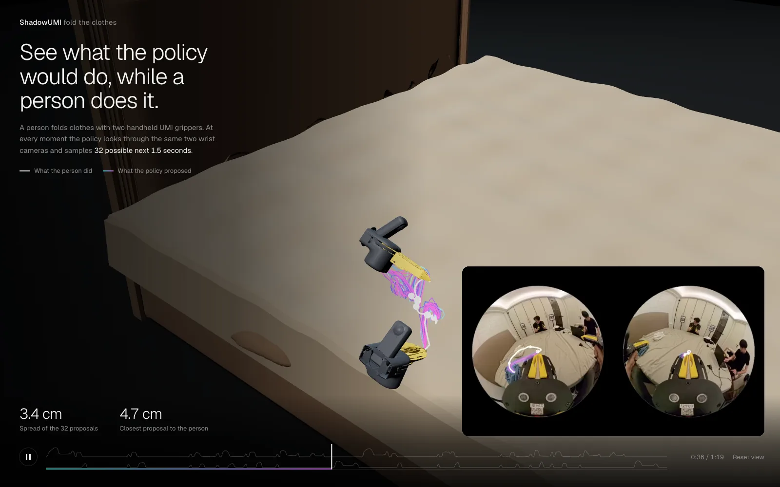 Open the episode in 3D ↗
Handheld collection devices such as UMI1 have made demonstration data cheap. A person with a pair of instrumented grippers can produce hours of usable bimanual data in a day, in homes, warehouses and kitchens no robot has visited. We operate this kind of collection at scale, and over the past year it has become clear that cost per hour is no longer the main limit on how good a policy gets. The limit is that every hour is collected open-loop. The person holding the gripper has no idea what the model already does well. Novel situations and situations the model mastered months ago receive the same care and the same time.
Robot learning has a standard fix for this: put the policy in control and let a human correct it2,3. That fix needs a robot. It also takes away the main advantage of handheld collection, which is that the person moves at their own speed, wherever they are, with no hardware to babysit. We wanted the same feedback without the robot.
Shadows are our answer. While the person works, the policy runs alongside them on the same two wrist cameras and draws its predictions into the scene: 32 sampled action chunks per hand, refreshed six times a second. The person does not follow the shadows. They do the task. But because the policy's proposals and the person's actual motion now share a frame and a clock, the episode records more than a trajectory. It records where the policy and the person agreed, where they disagreed, and how confident the model was when it was wrong.
Highlights
- Shadows run on standard handheld UMI hardware. Policy proposals line up with the reconstructed gripper path to within 0.3° and 0.2 cm after time alignment, so the comparison against the person's real motion is a measurement rather than an eyeball judgment.
- On a real folding episode, the spread of the policy's 32 samples is a poor signal of whether the policy is right. Near the end of the 1.67 s horizon the samples span 1.3 cm while the nearest one misses the person by 12 cm. The largest errors occur at ordinary spread.
- Matching the person's move against the scored proposals yields preference labels automatically. Those labels land where the value function is wrong, rather than spread evenly over the data. Disagreement within a value ensemble tells the policy where its coverage is thin.
- At an equal collection budget of 25 hours per task, policies trained on shadow-guided data reach 71% mean success on four household tasks, versus 49% for standard collection and 64% for standard collection at twice the budget.
What a shadow is
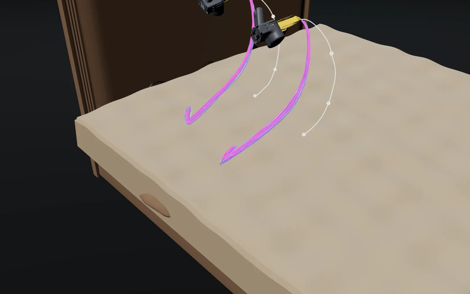
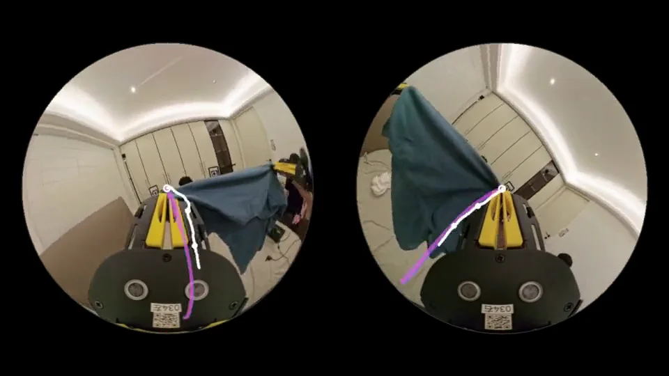
A shadow is a set of samples from the policy, drawn where the person can see them. Concretely, at each anchor frame (every fifth video frame, or 6 Hz) we take the latest image from both wrist cameras and the current gripper state and sample B = 32 action chunks from the policy π(at:t+H | ot). Each chunk covers H = 25 steps at 15 Hz for both hands, about 1.67 seconds. The predicted end-effector positions are placed in the same world frame as the reconstructed gripper trajectory and drawn two ways: as curves in the 3D scene, and projected back into the fisheye wrist images that the collector sees on their display.
The rendering is deliberately plain. Each of the 32 samples gets its own fixed hue from cyan to magenta, so a fan of identical colors means the samples have collapsed onto one another. The person's actual next 1.5 seconds is drawn in white, with ticks every half second. No sample is singled out as "the" prediction. The display is supposed to show what the policy might do, not tell the person what to do.
Making the shadow land in the right place
A shadow that is off by a few centimeters, or a fraction of a second, is worse than no shadow. The person sees disagreement that is really calibration error, and every label derived from it inherits the bias. Most of the engineering effort went here, not into the display.
Three things have to agree. The first is time. Wrist video, IMU and the reconstructed trajectory come from different clocks, and on our cameras the IMU stream starts 0.2–0.33 s before the first video frame. We estimate the offset per hand by aligning the camera trajectory against the IMU-integrated motion and reject any episode with a residual above threshold. The second is gravity. The direction of "up" estimated from the visual reconstruction must agree with the accelerometer. If it does not, every predicted trajectory tilts slightly, and the tilt grows with the horizon. The third is the tool point. The policy predicts the fingertip, and the camera sits 16 cm behind it, so a small orientation error at the camera becomes a positional error at the tip.
Alignment check, episode trk1021_094726 | Left hand | Right hand |
|---|---|---|
| Clock offset, video → trajectory | 3.62 s | 3.68 s |
| Rotation residual after alignment | 0.28° | 0.23° |
| Position residual after alignment | 0.23 cm | 0.17 cm |
| Gravity agreement, vision vs. IMU | 0.9° | |
| Camera-to-fingertip lever arm | 16.1 cm | |
Table 1. Alignment quality for the episode shown throughout this post. A 0.9° gravity error moves the fingertip by about 0.25 cm over the lever arm, well below the errors we analyze below.
Shadows also have to arrive on time. A prediction that shows up after the person has already moved is a historical note, not a shadow. The table below breaks down the end-to-end latency on our collection setup.
| Stage | Where it runs | Median | p95 |
|---|---|---|---|
| Capture, decode, rectify (2 cameras) | Collection edge box | 18 ms | 24 ms |
| Pose update (visual-inertial) | Collection edge box | 6 ms | 9 ms |
| Policy: 32 samples × 25 steps × 2 hands | Edge GPU | 92 ms | 118 ms |
| Value ensemble scoring (5 heads) | Edge GPU | 7 ms | 9 ms |
| Projection and render to wrist display | Handheld display | 8 ms | 12 ms |
| Glass to glass | 131 ms | 172 ms |
Table 2. Latency budget, measured over 1,000 anchors. At 6 Hz refresh, the shadow is never more than about 300 ms old, a fifth of its own horizon.
What one episode shows
Before using shadows to change how data is collected, we wanted to know what they show on their own. We took a folding policy trained on 420 hours of bimanual UMI data from 61 homes and ran it alongside a held-out episode: 80 seconds, 479 anchors, 32 samples each. At each anchor we compute two numbers per hand and average over hands:
- Spread: the mean distance of the 32 sample endpoints from their centroid. It measures how much the samples disagree with each other.
- Best-of-32 error: for each sample, the mean distance to the person's actual trajectory over the horizon; then the smallest of those 32 numbers. It measures how close the policy came to what the person did, giving it the benefit of the best sample.
Spread and best-of-32 error across the episode
centimeters · 479 anchors at 6 Hz · mean of both hands · click or drag to move through the episode
Two readings of this plot are tempting, and both are wrong. The first is that the policy is bad. A median best-of-32 error of 6.9 cm over a 1.67-second horizon of freehand folding, on an episode the model never saw, is within the range where the policy completes the task (it folds this shirt in 7 of 10 robot trials). The second reading is that spread is a usable proxy for error, so the policy could flag its own weak spots. Figure 4 shows why it cannot.
How error and spread grow with the prediction horizon
centimeters · averaged over all anchors and both hands
| Samples drawn, K | 1 | 2 | 4 | 8 | 16 | 32 |
|---|---|---|---|---|---|---|
| Best-of-K error (cm) | 8.64 | 8.39 | 8.19 | 8.02 | 7.88 | 7.75 |
Table 3. Best-of-K trajectory error on the episode, averaged over 50 random subsets per K. Each doubling of the sample count buys about 2%.
The samples are tightly clustered, and the cluster is often in the wrong place. Sampling a modern action head many times does not explore. It reports, with high precision, the single future the model currently believes in. That matters for everything downstream. Any scheme that uses sample diversity to decide where to collect more data will spend its effort where the task is genuinely ambiguous, such as choosing which corner of the shirt to grab. Those are exactly the moments the model handles well. It will spend nothing on the moments where the model is confidently wrong, because those look identical to the moments where it is confidently right.
Spread tells you how many ways the policy thinks the next second could go. It says nothing about whether any of them is right. Only the person knows that, and they already show it with their hands.
This is the observation the rest of the system is built on. The signal we need is not in the model. It is in the gap between the model and the person, measured at the moment the person makes a choice, and it costs nothing extra to collect because the person was going to make that choice anyway.
From watching to labeling
A shadow display by itself is a diagnostic. To make it a training signal, we add a second model and close a loop. Next to the policy we train an ensemble of M = 5 value heads V1…VM that score each proposal. On the display, a sample's color is no longer a fixed hue. It is the ensemble's mean score, from poor to good, and its width is the ensemble's disagreement. The person still does not follow anything. They do the task, and at the end of each round (one anchor interval) we compare what they did with what was on screen.
One choice, two kinds of supervision
Let τ1…τB be the proposals at an anchor, and let τ* be the proposal closest to the person's actual motion over the round. Every proposal that differs meaningfully from τ* (by more than 4 cm at the horizon) becomes the losing side of a preference pair. The value ensemble is trained with a Bradley–Terry loss4 on these pairs, alongside ordinary temporal-difference targets from the episode:
The same motion is a behavior-cloning target for the policy, exactly as in standard collection. So far this is a modest gain: one round produces up to 31 comparisons in addition to the demonstration. The more useful property is where the comparisons fall.
Before the person moves, the ensemble has already ranked the proposals. If its top choice τVF = argmaxj μ(τj) is not the one the person chose, the pair (τ*, τVF) is a correction placed exactly on a value-function mistake. Uniformly sampled preference queries waste most of their budget confirming what the critic already knows. Here the label distribution follows the critic's errors automatically, with no query selection step, because the person only disagrees with the display when the display is wrong.
The mechanics are easier to see in a reduced setting than on a folding shirt, so the next four figures use a toy version of the loop. A gripper on a top-down table has to go around a box to reach a cup. The policy starts out pointing straight at the cup, through the box. Each of the five value heads starts from a distance-to-cup prior plus its own random bumps, so at first the ensemble rates the rollouts that crash into the box highly. A simulated expert walks the shortest path with some wobble. Everything below runs live in the page, with the same update rules as Eqs. 1 and 2.
One round, slowed down
Disagreement as coverage
The ensemble also gives the policy something the sample spread could not: an estimate of whether a state has been seen. Every ensemble member starts with its own random bias. Where the person has worked and labeled, all members are pulled toward the same targets and their disagreement σV(s) shrinks. Where nobody has been, each member keeps its own prior5,6. The policy uses this in two ways. Its sampling width at a state scales with σV, so shadows fan out where coverage is thin. And it only learns from the critic's advantages where the ensemble agrees:
The term LAW is an advantage-weighted regression toward the proposals with the highest lower confidence bound μ − 1.5σ. In covered states, the policy can improve against the critic between human visits. In uncovered states it falls back to imitation and waits for data.
The same collection run at four moments
Where corrections land
The claim that labels follow the critic's errors can be checked directly in the toy. Figure 7 runs the loop live, with the value function's current error shaded underneath. Each round that ends in a correction leaves a ring, and each round that ends in agreement leaves a faint dot. The rings gather on the darkest shading, and the shading under them fades within a few rounds. Over three seeds of four minutes each, rounds that produced a correction carried 3.7–5.0× the value-function error of rounds that did not.
Corrections against the value function's error
Value-function error is the mean |ensemble score − true return| over the round's six rollouts, at the moment they were shown. Running averages over recent rounds.
The whole loop
Figure 8 puts the pieces together and hands you the gripper. In human-guided mode, agreement rises and disagreement falls as labels accumulate, and the policy's success from seven fixed starting points climbs as it learns the way around the box. Switch to autonomous mode after a minute or two. From covered starting points the policy reaches the cup on its own. Elsewhere it collides, and the low-coverage tag appears before it does.
Experiments
We compared three ways of spending the same collection budget, with the same collectors, devices and homes.
- Standard UMI. Collectors perform the task as usual. No display.
- Shadows only. Collectors see the policy's 32 samples in fixed hues, with no value scoring. The policy is retrained on accumulated data every 5 hours, so the shadows improve during collection. Data are used for behavior cloning only.
- ShadowUMI. The full loop: scored and width-coded shadows, preference labels from Eq. 1, and policy updates from Eq. 2.
Every policy uses the same architecture and the same pretraining checkpoint, and is fine-tuned only on the data its arm collected. Success rates come from 20 trials per task on a bimanual robot with UMI-matched grippers, in two held-out homes, scored blind by an evaluator who did not know which arm produced the checkpoint.
| Task | Standard UMI 25 h | Shadows only 25 h | ShadowUMI 25 h | Standard UMI 50 h |
|---|---|---|---|---|
| Fold a T-shirt (bimanual) | 35 | 45 | 60 | 50 |
| Flatten a bed sheet (bimanual) | 45 | 55 | 70 | 60 |
| Hang a towel on a rail | 55 | 65 | 75 | 70 |
| Pack shoes into a box | 60 | 70 | 80 | 75 |
| Mean | 49 | 59 | 71 | 64 |
Table 4. Task success (%) at equal collection hours. ShadowUMI at 25 hours exceeds standard collection at 50 hours on every task.
Success rate vs. collection hours, fold a T-shirt
% of 20 trials · same collectors and homes in every arm
The shape of Figure 9 says something about when shadows help. Early in collection the policy is wrong almost everywhere, so a correction is no more informative than the demonstration itself. The gain appears once the policy is right most of the time. Then the person's disagreements become rare and specific, and each one is worth much more than an average minute of demonstration. In other words, shadows do not replace the first hours of data. They change the value of every hour after that.
Where the labels go
Value function vs. collector over the course of collection
% of rounds · fold a T-shirt · rolling 1-hour window
Ablations
| Fold a T-shirt, 25 h | Success | VF agrees with collector | Labels on VF errors |
|---|---|---|---|
| ShadowUMI (full) | 60 | 77 | 23 |
| − preference loss (TD only) | 50−10 | 62 | — |
| − value scoring on display | 48−12 | 66 | 19 |
| − disagreement-scaled sampling width | 53−7 | 74 | 21 |
| − confidence gate in Eq. 2 (w = 1) | 41−19 | 75 | 22 |
| Single value head instead of 5 | 51−9 | 70 | 20 |
Table 5. All values in %. Removing the confidence gate hurts most: without it, the policy follows the critic's advantages into states the critic has never seen and drifts below the shadows-only baseline. The display matters too. Collectors with an unscored display disagree with the policy about as often, but their disagreements are less often at critic errors.
Do collectors copy the shadow?
The most obvious risk of showing a person the model's predictions is that they start following them. Then the data stops correcting the model and only confirms it. We measured this directly by alternating shadows on and off in 10-minute blocks for the same collectors.
| Per collector-hour | Shadows off | Shadows on |
|---|---|---|
| Episodes completed | 21.4 | 19.8 |
| Median episode length | 74 s | 79 s |
| Distance from policy mean, median over anchors | 8.6 cm | 7.9 cm |
| Rounds where collector matched the VF's top choice | 71% | 77% |
| Time with eyes on the display | — | 11% |
| Self-reported workload (NASA-TLX, 0–100) | 38 | 41 |
Table 6. Collectors move about 8% closer to the policy's mean when shadows are visible. That is a measurable anchoring effect. They still part ways with the value function's top choice in roughly one round in four, and those rounds carry most of the labels' value. Throughput falls by 7%.
Two changes to the protocol kept anchoring in check. Collectors are told that the shadow is the model's guess and that disagreeing with it is the point. And the display shows nothing during the first 0.3 s of each round, so the person commits to a direction before the newest shadow appears. We consider anchoring the main open problem with this approach and continue to measure it in every collection run.
What changes when collection closes the loop
The usual picture of data collection for robot learning is a pipeline: people produce demonstrations, a training job consumes them, an evaluation tells you whether to collect more. Shadows move part of the evaluation into collection itself. Every round is a small comparison between the current model and a person who knows the task, made at the person's natural pace, with no robot in the loop. Three consequences follow.
Collection effort can be allocated. Because disagreement is measured per state, we can see in near real time which parts of a task the model has learned and send collectors to the parts it has not, such as a particular fabric, a particular step of a fold, or a particular kind of room. In our current runs, about 40% of collector time is now directed by these coverage maps.
The handheld device becomes a source of on-policy information without being on-policy. DAgger-style methods get their power from querying the expert in states the learner visits2. Shadows query the expert about actions the learner proposes, in states the expert visits. That is weaker. The person never has to rescue the policy from a state it drove into. But it covers the large share of policy errors that are wrong choices in ordinary states, and it is available everywhere handheld collection already runs.
The person stays the authority. Nothing in the loop asks a collector to rate, rank or annotate anything. The labels come from what they do with their hands, which is the one thing they do reliably and fast. We think this matters more than any part of the model. Preference labels from people who are thinking about the labels are noisy and slow. Preference labels from people who are thinking about the shirt are neither.
Limitations
- Shadows show kinematics only. A proposal can have the right path and the wrong grip force, and nothing on the display reveals it.
- The analysis in Figures 2–4 comes from a single episode. The experimental results cover four tasks and a limited number of collectors and homes.
- The value ensemble learns the person's preferences, including their mistakes. The toy in Figure 8 makes this easy to demonstrate. In practice we rely on many collectors disagreeing in different ways.
- The preference threshold δ and the confidence constants in Eq. 2 were tuned on one task and reused for the others without re-tuning.
Appendix: how the episode figures are computed
The episode is session_trk1021_094726: 2,395 frames at 30 fps, two grippers. Proposals are stored at 479 anchors (every 5 frames) as 32 samples × 2 hands × 26 points (the current pose plus 25 future steps, 2 frames apart). For anchor t, hand h, sample b: spread is the mean over b of ‖pbend − p̄end‖; best-of-32 error is minb of the mean over steps k of ‖pbk − xt+2k‖, where x is the reconstructed fingertip path. Both are averaged over the two hands. Anchors whose horizon runs past the end of the episode are dropped from Figure 4 and Table 3 (469 remain). The same numbers appear live in the episode viewer.
References
- C. Chi, Z. Xu, C. Pan, E. Cousineau, B. Burchfiel, S. Feng, R. Tedrake, S. Song. Universal Manipulation Interface: In-the-Wild Robot Teaching Without In-the-Wild Robots. RSS 2024.
- S. Ross, G. Gordon, D. Bagnell. A Reduction of Imitation Learning and Structured Prediction to No-Regret Online Learning. AISTATS 2011.
- M. Kelly, C. Sidrane, K. Driggs-Campbell, M. Kochenderfer. HG-DAgger: Interactive Imitation Learning with Human Experts. ICRA 2019.
- P. Christiano, J. Leike, T. Brown, M. Martic, S. Legg, D. Amodei. Deep Reinforcement Learning from Human Preferences. NeurIPS 2017.
- B. Lakshminarayanan, A. Pritzel, C. Blundell. Simple and Scalable Predictive Uncertainty Estimation using Deep Ensembles. NeurIPS 2017.
- I. Osband, C. Blundell, A. Pritzel, B. Van Roy. Deep Exploration via Bootstrapped DQN. NeurIPS 2016.
Citation
@misc{crobotia2026shadows,
  title  = {Shadows: Letting the Person Collecting the Data See What the Policy Would Do},
  author = {Crobotia Research},
  year   = {2026},
  url    = {https://shadow.crobotia.com}
}